Introduction

This article is for search practitioners who want to achieve a deep understanding of the ranking functions TF-IDF and BM25 (also called “similarities” in Lucene). If you’re like many practitioners, you’re already familiar with TF-IDF, but when you first saw the complicated BM25 formula, you thought “maybe later.” Now is the time to finally understand it! You’ve probably heard that BM25 is similar to TF-IDF but works better in practice. This article will show you precisely how BM25 builds upon TF-IDF, what its parameters do, and why it is so effective. If you’d rather skip over the math and work with practical examples that demonstrate BM25’s behaviors, check out our companion article on Understanding Scoring Through Examples.

Reviewing TF-IDF

Let’s review TF-IDF by trying to develop it from scratch. Imagine we’re building a search engine. Assume we’ve already got a way to find the documents that match a user’s search. What we need now is a ranking function that will tell us how to order those documents. The higher a document’s score according to this function, the higher up we’ll place it in the list of results that we return to the user.

The goal of TF-IDF and similar ranking functions is to reward relevance. Say a user searches for the term “dogs.” If Document 1 is more relevant to the subject of dogs than Document 2, then we want the score of Document 1 to be higher than the score of Document 2, so we’ll show the better result first and the user will be happy. How much higher does Document 1’s score have to be? It doesn’t really matter, as long as the score order matches the relevance order.

You might feel a little shocked by the audacity of what we’re attempting to do: we’re going to try to judge the relevance of millions or billions of documents using a mathematical function, without knowing anything about the person who’s doing the search, and without actually reading the documents and understanding what they’re about! How is this possible?

We’ll make a simple but profoundly helpful assumption. We’ll assume that the more times a document contains a term, the more likely it is to be about that term. That’s to say, we’ll use term frequency (TF), the number of occurrences of a term in a document, as a proxy for relevance. This one assumption creates a path for us to solve a seemingly impossible problem using simple math. Our assumption isn’t perfect, and it goes very wrong sometimes, but it works often enough to be useful. So from here on, we’ll view term frequency as a good thing — a thing we want to reward.

TF-IDF: Attempt 1

As a starting point for our ranking function, let’s do the simplest, easiest thing possible. We’ll set the score of a document equal to its term frequency. If we’re searching for a term T and evaluating the relevance of a document D, then:

score(D, T) = termFrequency(D, T)

When a query has multiple terms, like “dogs and cats,” how should we handle that? Should we try to analyze the relationships between the various terms and then blend the per-term scores together in a complex way? Not so fast! The simplest approach is to just add the scores for each term together. So we’ll do that, and hope for the best. If we have a multi-term query Q, then we’ll set:

score(D, Q) = sum over all terms T in Q of score(D, T)

How well does our simple ranking function work? Unfortunately, it’s got some problems:

1) Longer documents are given an unfair advantage over shorter ones because they have more space to include more occurrences of a term, even though they might not be more relevant to the term. Let’s ignore this problem for now.

2) All terms in a query are treated equally, with no consideration for which ones are more meaningful or important. When we sum the scores for each term together, insignificant terms like “and” and “the” which happen to be very frequent will dominate the combined score. Say you search for “elephants and cows.” Perhaps there’s a single document in the index that includes all three terms (“elephants”, “and”, “cows”), but instead of seeing this ideal result first, you see the document that has the most occurrences of “and” — maybe it has 10,000 of them. This preference for filler words is clearly not what we want.

TF-IDF: Attempt 2

To prevent filler words from dominating, we need some way of judging the importance of the terms in a query. Since we can’t encode an understanding of natural language into our scoring function, we’ll try to find a proxy for importance. Our best bet is rarity. If a term doesn’t occur in most documents in the corpus, then whenever it does occur, we’ll guess that this occurrence is significant. On the other hand, if a term occurs in most of the documents in our corpus, then the presence of that term in any particular document will lose its value as an indicator of relevance.

So high term frequency is a good thing, but its goodness is offset by high document frequency (DF) — the number of documents that contain the term — which we’ll think of as a bad thing.

To update our function in a way that rewards term frequency but penalizes document frequency, we could try dividing TF by DF:

score(D, T) = termFrequency(D, T) / docFrequency(T)

What’s wrong with this? Unfortunately, DF by itself tells us nothing. If DF for the term “elephant” is 100, then is “elephant” a rare term or a common term? It depends on the size of the corpus. If the corpus contains 100 documents, “elephant” is common, if it contains 100,000 documents, “elephant” is rare.

TF-IDF: Attempt 3

Instead of looking at DF by itself, let’s look at N/DF, where N is the size of the search index or corpus. Notice how N/DF is low for common terms (100 occurrences of “elephant” in a corpus of size 100 would give N/DF = 1), and high for rare ones (100 occurrences of “elephant in a corpus of size 100,000 would give N/DF = 1000). That’s exactly what we want: matches for common terms should get low scores, matches for rare terms should get high ones. Our improved formula might go like this:

score(D, T) = termFrequency(D, T) * (N / docFrequency(T))

We’re doing better, but let’s take a closer look at how N/DF behaves. Say we have 100 documents and “elephant” occurs in 1 of them while “giraffe” occurs in 2 of them. Both terms are similarly rare, but elephant’s N/DF value would come out to 100 and giraffe’s would be half that, at 50. Should a match for giraffe get half the score of match for elephant just because giraffe’s document frequency is one higher then elephant’s? The penalty for one additional occurrence of the word in the corpus seems too high. Arguably, if we have 100 documents, it shouldn’t make much of a difference whether a term’s DF is 1, 2, 3, or 4 .

TF-IDF: Attempt 4

As we’ve seen, when DF is in a very low range, small differences in DF can have a dramatic impact on N/DF and hence on the score. We might like to smooth out the decline of N/DF when DF is in the lowest end of its range. One way to do this is to take the log of N/DF. If we wanted, we could try to use a different smoothing function here, but log is straightforward and it does what we want. This chart compares N/DF and log(N/DF) assuming N=100:

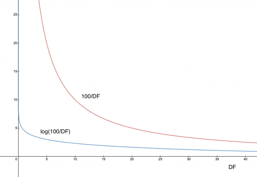
Let’s call log(N/DF) the inverse document frequency (IDF) of a term. Our ranking function can now be expressed as TF * IDF or:

score(D, T) = termFrequency(D, T) * log(N / docFrequency(T))

We’ve arrived at the traditional definition of TF-IDF and even though we made some bold assumptions to get here, the function works pretty well in practice: it has gathered a long track record of successful application in search engines. Are we done or could we do even better?

Developing BM25

As you might have guessed, we’re not ready to stop at TF-IDF. In this section, we’ll build the BM25 function, which can be seen as an improvement on TF-IDF. We’re going to keep the same structure of the TF * IDF formula, but we’ll replace the TF and IDF components with refinements of those values.

Step 1: Term Saturation

We’ve been saying that TF is a good thing, and indeed our TF-IDF formula rewards it. But if a document contains 200 occurrences of “elephant,” is it really twice as relevant as a document that contains 100 occurrences? We could argue that if “elephant” occurs a large enough number of times, say 100, the document is almost certainly relevant, and any further mentions don’t really increase the likelihood of relevance. To put it a different way, once a document is saturated with occurrences of a term, more occurrences shouldn’t a have a significant impact on the score. So we’d like a way to control the contribution of TF to our score. We’d like this contribution to increase fast when TF is small and then increase more slowly, approaching a limit, as TF gets very big.

One common way to tame TF is to take the square root of it, but that’s still an unbounded quantity. We’d like to do something more sophisticated. We’d like to put a bound on TF’s contribution to the score, and we’d like to be able to control how rapidly the contribution approaches that bound. Wouldn’t it be nice if we had a parameter k that could control the shape of this saturation curve? That way, we’d be able to experiment with different values of k and see what works best for a particular corpus.

To achieve this, we’ll pull out a trick. Instead of using raw TF in our ranking formula, we’ll use the value:

TF / (TF + k)

If k is set to 1, this would generate the sequence 1/2, 2/3, 3/4, 4/5, 5/6 as TF increases 1, 2, 3, etc. Notice how this sequence grows fast in the beginning and then more slowly, approaching 1 in smaller and smaller increments. That’s what we want. Now if we change k to 2, we’d get 1/3, 2/4, 3/5, 4/6 which grows a little more slowly. Here’s a graph of the formula TF/(TF + k) for k = 1, 2, 3, 4:

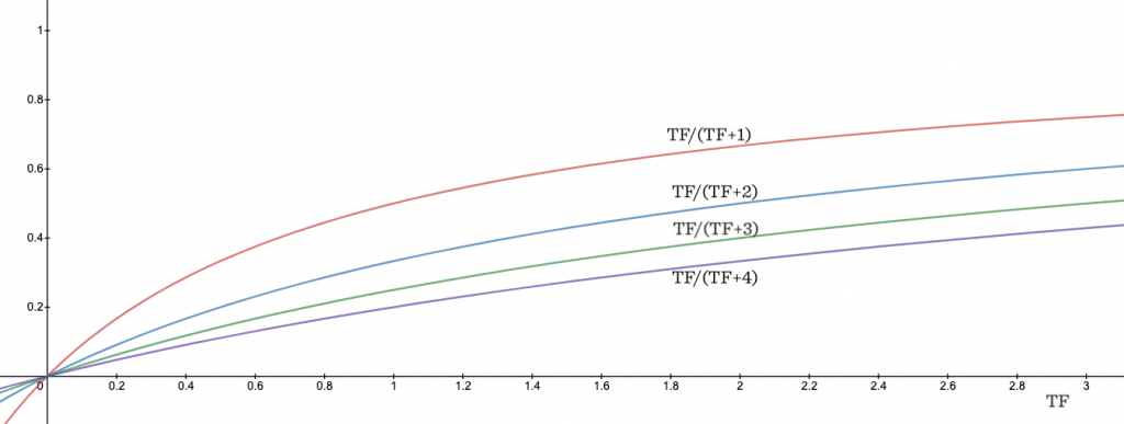
This TF/(TF + k) trick is really the backbone of BM25. It lets us control the contribution of TF to the score in a tunable way.

Aside: Term Saturation and Multi-Term Queries

A fortunate side-effect of using TF/(TF + k) to account for term saturation is that we end up rewarding complete matches over partial ones. That’s to say, we reward documents that match more of the terms in a multi-term query over documents that have lots of matches for just one of the terms.

Let’s say that “cat” and “dog” have the same IDF values. If we search for “cat dog” we’d like a document that contains one instance of each term to do better than a document that has two instances of “cat” and none of “dog.” If we were using raw TF they’d both get the same score. But let’s do our improved calculation assuming k=1. In our “cat dog” document, “cat” and “dog” each have TF=1, so each are going to contribute TF/(TF+1) = 1/2 to the score, for a total of 1. In our “cat cat” document, “cat” has a TF of 2, so it’s going to contribute TF/(TF+1) = 2/3 to the score. The “cat dog” document wins, because “cat” and “dog” contribute more when each occurs once than “cat” contributes when it occurs twice.

Assuming the IDF of two terms is the same, it’s always better to have one instance of each term than to have two instances of one of them.

Step 2: Document Length

Now let’s go back to the problem we skipped over when we were first building TF-IDF: document length. If a document happens to be really short and it contains “elephant” once, that’s a good indicator that “elephant” is important to the content. But if the document is really, really long and it mentions elephant only once, the document is probably not about elephants. So we’d like to reward matches in short documents, while penalizing matches in long documents. How can we achieve this?

First, we’ve got to decide what it means for a document to be short or long. We need a frame of reference, so we’ll use the corpus itself as our frame of reference. A short document is simply one that is shorter than average for the corpus.

Let’s go back to our TF/(TF + k) trick. Of course as k increases, the value of TF/(TF + k) decreases. To penalize long documents, we can adjust k up if the document is longer than average, and adjust it down if the document is shorter than average. We’ll achieve this by multiplying k by the ratio dl/adl. Here, dl is the document’s length, and adl is the average document length across the corpus.

When a document is of average length, dl/adl =1, and our multiplier doesn’t affect k at all. For a document that’s shorter than average, we’ll be multiplying k by a value between 0 and 1, thereby reducing it, and increasing TF/(TF+k). For a document that’s longer than average, we’ll be multiplying k by a value greater than 1, thereby increasing it, and reducing TF/(TF+k). The multiplier also puts us on a different TF saturation curve. Shorter documents will approach a TF saturation point more quickly while longer documents will approach it more gradually.

Step 3: Parameterizing Document Length

In the last section, we updated our ranking function to account for document length, but is this always a good idea? Just how much importance should we place on document length in any particular corpus? Might there be some collections of documents where length matters a lot and some where it doesn’t? We might like to treat the importance of document length as a second parameter that we can experiment with.

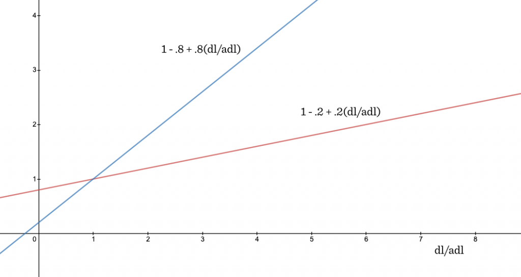
We’re going to achieve this tunability with another trick. We’ll add a new parameter b into the mix (it must be between 0 and 1). Instead of multiplying k by dl/adl as we were doing before, we’ll multiply k by the following value based on dl/adl and b:

1 – b + b*dl/adl

What does this do for us? You can see if b is 1, we get (1 – 1 + 1*dl/adl) and this reduces to the multiplier we had before, dl/adl. On the other hand, if b is 0, the whole thing becomes 1 and document length isn’t considered at all. As b is cranked up from 0 towards 1, the multiplier responds more quickly to changes in dl/adl. The chart below shows how our multiplier behaves as dl/adl grows, when b=.2 versus when b=.8.

Recap: Fancy TF

To recap, we’ve been working modifying the TF term in TF * IDF so that it’s responsive to term saturation and document length. To account for term saturation, we introduced the TF/(TF + k) trick. To account for document length, we added the (1 – b + b*dl/adl) multiplier. Now, instead of using raw TF in our ranking function, we’re using this “fancy” version of TF:

TF/(TF + k*(1 - b + b*dl/adl)) 

Recall that k is the knob that control the term saturation curve, and b is the knob that controls the importance of document length.

Indeed, this is the version of TF that’s used in BM25. And congratulations: if you’ve followed this far, you now understand all the really interesting stuff about BM25.

Step 4: Fancy or Not-So-Fancy IDF

We’re not done just yet though, we have to return to the way BM25 handles document frequency. Earlier, we had defined IDF as log(N/DF), but BM25 defines it as:

log((N - DF + .5)/(DF + .5)) 

Why the difference?

As you may have observed, we’ve been developing our scoring function through a set of heuristics. Researchers in the field of Information Retrieval have wanted to put ranking functions on a more rigorous theoretical footing so they can actually prove things about their behavior rather than just experimenting and hoping for the best. To derive a theoretically sound version of IDF, researchers took something called the Robertson-Spärck Jones weight, made a simplifying assumption, and came up with log (N-DF+.5)/(DF+.5). We’re not going to go into the details, but we’ll just focus on the practical significance of this flavor of IDF. The .5’s don’t really do much here, so let’s just consider log (N-DF)/DF, which is sometimes referred to as “probabilistic IDF.” Here we compare our vanilla IDF with probabilistic IDF where N=10.

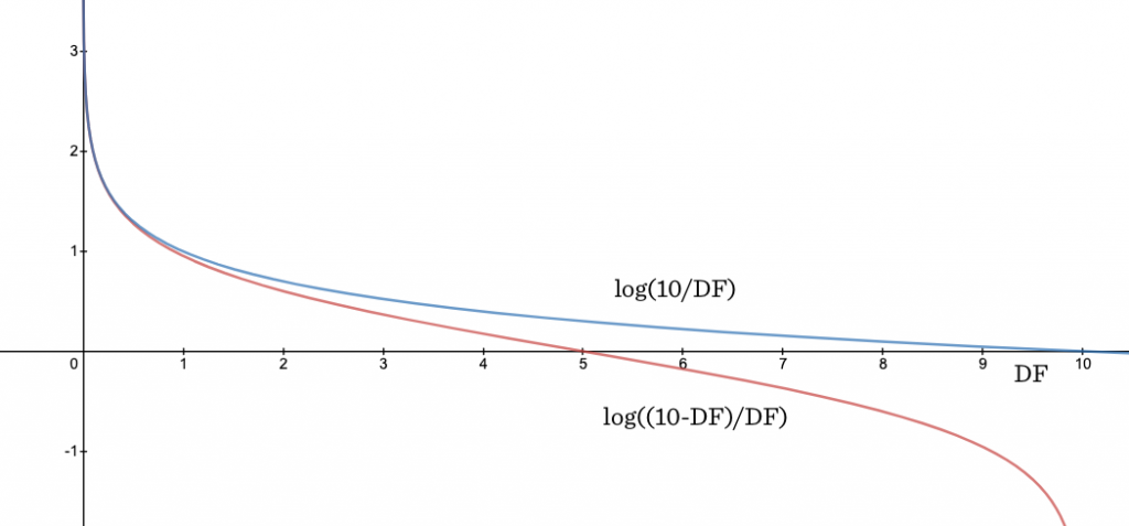
You can see that probabilistic IDF takes a sharp drop for terms that are in most of the documents. This might be desirable because if a term really exists in 98% of the documents, it’s probably a stopword like “and” or “or” and it should get much, much less weight than a term that’s very common, like in 70% of the documents, but still not utterly ubiquitous.

The catch is that log (N-DF)/DF is negative for terms that are in more than half of the corpus. (Remember that the log function goes negative on values between 0 and 1.) We don’t want negative values coming out of our ranking function because the presence of a query term in a document should never count against retrieval — it should never cause a lower score than if the term was simply absent. In order to prevent negative values, Lucene’s implementation of BM25 adds a 1 like this:

IDF = log (1 + (N - DF + .5)/(DF + .5))

This 1 might seem like an innocent modification but it totally changes the behavior of the formula! If we forget again about those pesky .5’s, and we note that adding 1 is the same as adding DF/DF, you can see that the formula reduces to the vanilla version of IDF that we used before: log (N/DF).

log (1 + (N - DF + .5)/(DF + .5)) ≈
log (1 + (N - DF)/DF ) =
log (DF/DF + (N - DF)/DF) = 
log ((DF + N - DF)/DF) = 
log (N/DF)

So although it looks like BM25 is using a fancy version of IDF, in practice (as implemented in Lucene) it’s basically using the same old version of IDF that’s used in traditional TF/IDF, without the accelerated decline for high DF values.

Cashing In

We’re ready to cash in on our new understanding by looking at the explain output from a Lucene query. You’ll see something like this:

“score(freq=3.0), product of:”

“idf, computed as log(1 + (N — n + 0.5) / (n + 0.5)) from:”

“tf, computed as freq / (freq + k1 * (1 — b + b * dl / avgdl)) from:”

We’re finally prepared to understand this gobbledygook. You can see that Lucene is using a TF*IDF product where TF and IDF have their special BM25 definitions. Lowercase n means DF here. The IDF term is the supposedly fancy version that turns out to be the same as traditional IDF, N/n.

The TF term is based on our saturation trick: freq/(freq + k). The use of k1 instead of k in the explain output it historical — it comes from a time when there was more than one k in the formula. What we’ve been calling raw TF is denoted as freq here.

We can see that k1 is multiplied by a factor that penalizes above-average document length while rewarding below-average document length: (1-b + b *dl/avgdl). What we’ve been calling adl is denoted as avgdl here.

And of course we can see that there are parameters, which are set to k=1.2 and b = .75 in Lucene by default. You probably won’t need to tweak these, but you can if you want.

In summary, simple TF-IDF rewards term frequency and penalizes document frequency. BM25 goes beyond this to account for document length and term frequency saturation. 

It’s worth noting that before Lucene introduced BM25 as the default ranking function as of version 6, it implemented TF-IDF through something called the Practical Scoring Function, which was a set of enhancements (including “coord” and field length normalization) that made TF-IDF more like BM25. So the behavior difference one might have observed when Lucene made the switch to BM25 was probably less dramatic than it would have been if Lucene had been using pure TF-IDF all along. In any case, the consensus is that BM25 is an improvement, and now you can see why.

If you’re a search engineer, the Lucene explain output is the most likely place where you’ll encounter the details of the BM25 formula. However, if you delve into theoretical papers or check out the Wikipedia article on BM25, you’ll see it written out as an equation like this:

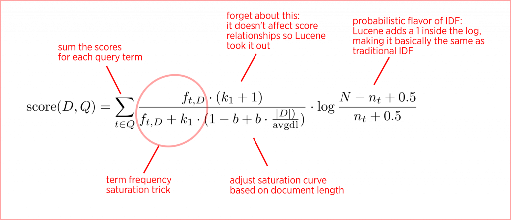
Hopefully this tour has made you more comfortable with how the two most popular search ranking functions work. Thanks for following along!

Further Reading

This article follows in the footsteps of some other great tours of BM25 that are out there. These two are highly recommended:

BM25 The Next Generation of Lucene Relevance by Doug Turnbull

Practical BM25 – Part 2: The BM25 Algorithm and its Variables by Shane Connelly

There are many theoretical treatments of ranking out there. A good starting place is “The Probabilistic Relevance Framework: BM25 and Beyond” by Robertson and Zaragosa. 

See also the paper “Okapi at TREC-3” where BM25 was first introduced.